Overview
Teaching: 10 min Exercises: 5 minQuestions
What is groupby processing and in what cases is it useful for scientific analysis of multidimensional arrays?
Objectives
Learn the concepts of split/apply/combine and experimenting with xarray groupby processing
GroupBy processing
We often want to build a time series of change from spatially distributed data. For example, suppose we need to plot a time series of the global average air temperature across the entire period of our climate data record. To accomplish this, xarray has powerful GroupBy processing tools, similar to the well known GROUP BY processing used in SQL. In all cases we split the data, apply a function to independent groups, and combine back into a known data structure.
Groupby processing: split
We can groupby the name of a variable or coordinate. Either returns an xarray groupby object:
ds[‘t2m’].groupby(‘time’)
Groupby processing: apply
Next we apply a function across the groupings set up in the xarray groupby process. When providing a single dimension to the groupby command, apply processes the function across the remaining dimensions. We could do the following:
def mean(x):
    return x.mean()

ds['t2m'].groupby('time').apply(mean).plot()
However, groupby objects have convenient shortcuts:
ds['t2m'].groupby('time').mean().plot()
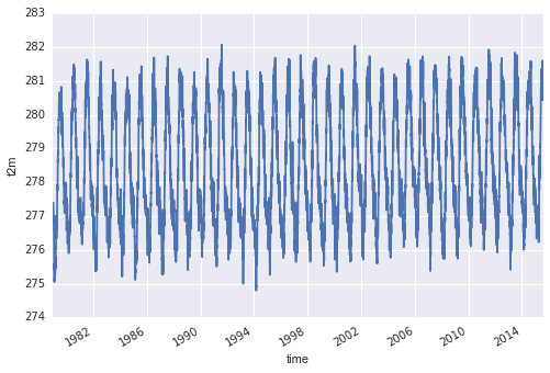
This is the daily global average air temperature during the entire period of record.
groupby
Above we calculated daily global averages. Try to calculate the global annual average instead, and plot the results as a 1-D time series.
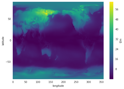
As a final example, here’s a very interesting way to explore seasonal variations in temperature data using xarray:
ds_by_season = ds['t2m'].groupby('time.season').mean('time')
t2m_range = abs(ds_by_season.sel(season='JJA') - ds_by_season.sel(season='DJF'))
t2m_range.plot()
Key Points
xarray provides Pandas-like methods for performing data aggregation over defined groupings in the data