Overview

Teaching: 15 min
Exercises: 0 min

Questions

• What is a raster?

• What are the main attributes of raster data?

Objectives

• Understand the raster data model

• Describe the strengths and weaknesses of storing data in raster format.

• Distinguish between continuous and categorical raster data and identify types of datasets that would be stored in each format.

Data Structures: Raster and Vector

The two primary types of geospatial data are raster and vector data. Vector data structures represent specific features on the Earth’s surface, and assign attributes to those features. Raster data is stored as a grid of values which are rendered on a map as pixels. Each pixel value represents an area on the Earth’s surface.

About Raster Data

Raster data is any pixelated (or gridded) data where each pixel is associated with a specific geographical location. The value of a pixel can be continuous (e.g. elevation) or categorical (e.g. land use).

If this sounds familiar, it is because this data structure is very common: it’s how we represent any digital image. A geospatial raster is only different from a digital photo in that it is accompanied by spatial information that connects the data to a particular location. This includes the raster’s extent and cell size, the number of rows and columns, and its coordinate reference system (or CRS).

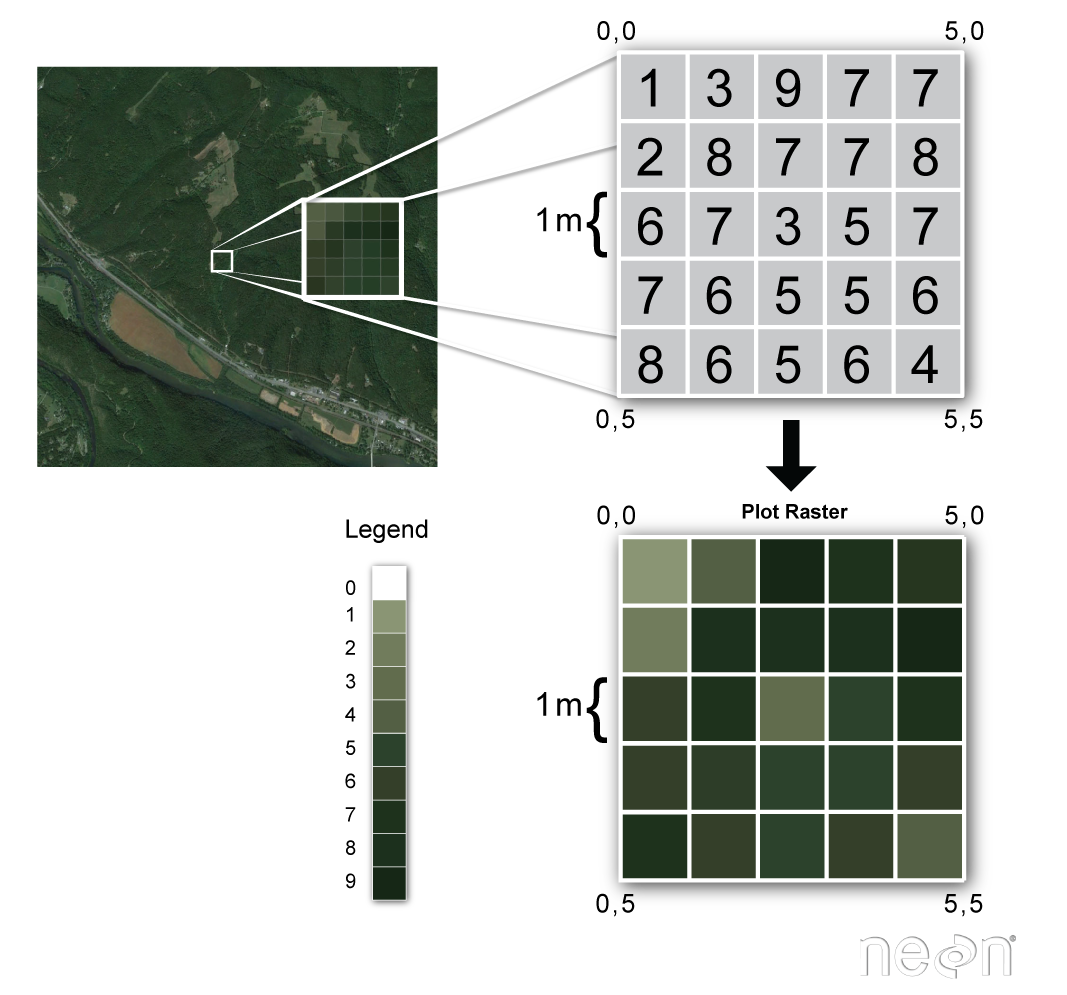
Source: National Ecological Observatory Network (NEON)

In the 1950’s raster graphics were noted as a faster and cheaper (but lower-resolution) alternative to vector graphics.

Some examples of continuous rasters include:

1. Orthorectified multispectral imagery such as those acquired by Landsat or MODIS sensors
2. Digital Elevation Models (DEMs) such as ASTER GDEM
3. Maps of canopy height derived from LiDAR data.

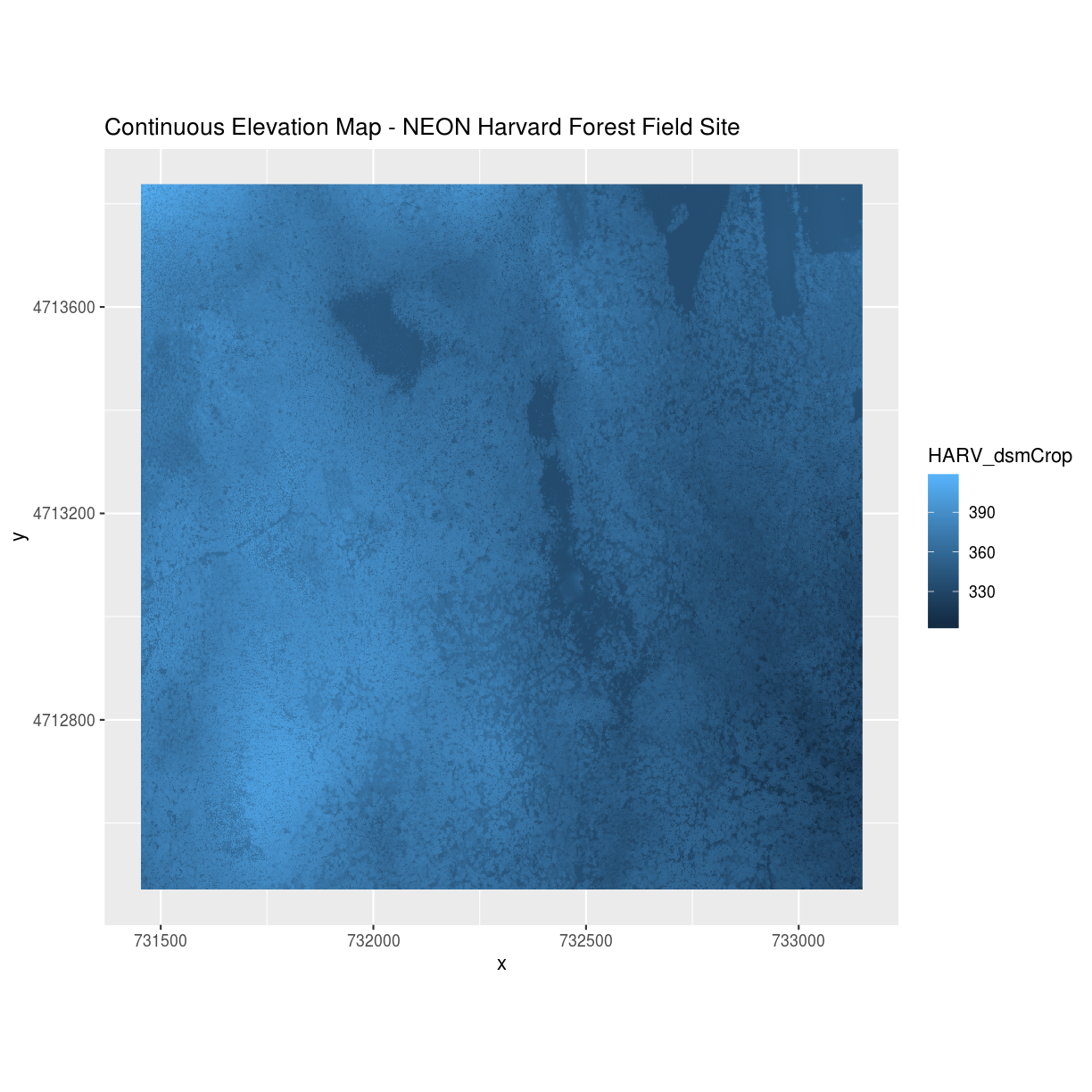
A map of elevation for Harvard Forest derived from the NEON AOP LiDAR sensor is below. Elevation is represented as continuous numeric variable in this map. The legend shows the continuous range of values in the data from around 300 to 420 meters.

Some rasters contain categorical data where each pixel represents a discrete class such as a landcover type (e.g., “forest” or “grassland”) rather than a continuous value such as elevation or temperature. Some examples of classified maps include:

1. Landcover / land-use maps.
2. Tree height maps classified as short, medium, and tall trees.
3. Snowcover masks (binary snow or no snow)

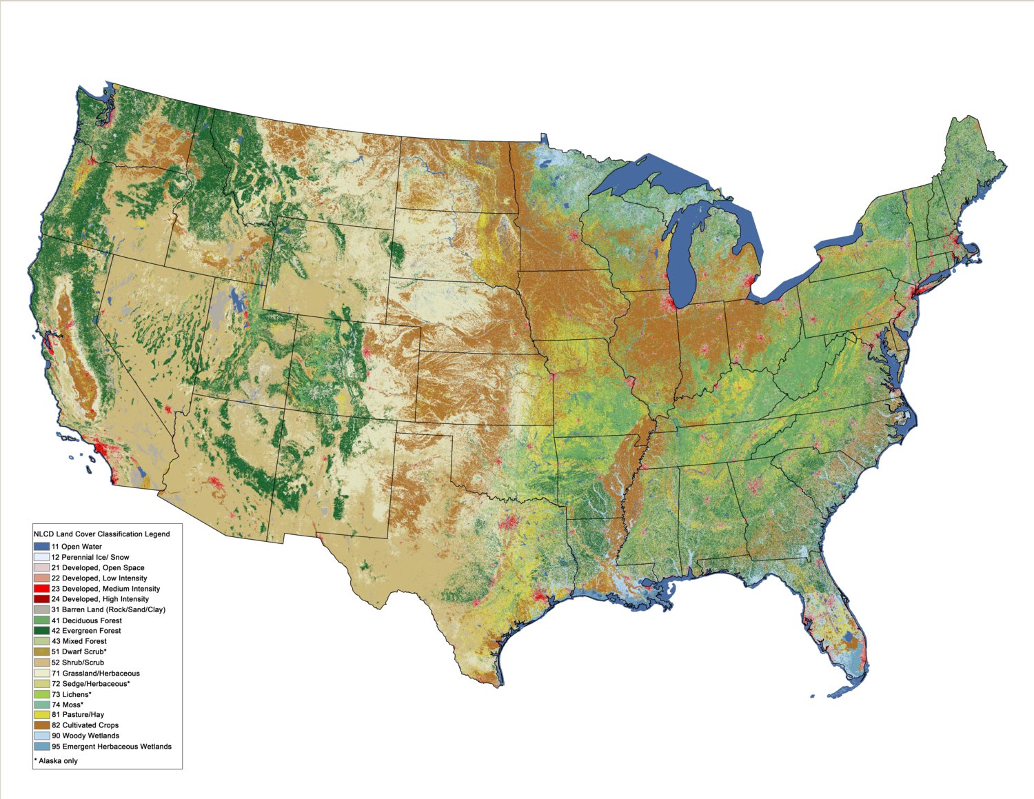
The following map shows the contiguous United States with landcover as categorical data. Each color is a different landcover category. (Source: Homer, C.G., et al., 2015, Completion of the 2011 National Land Cover Database for the conterminous United States-Representing a decade of land cover change information. Photogrammetric Engineering and Remote Sensing, v. 81, no. 5, p. 345-354)

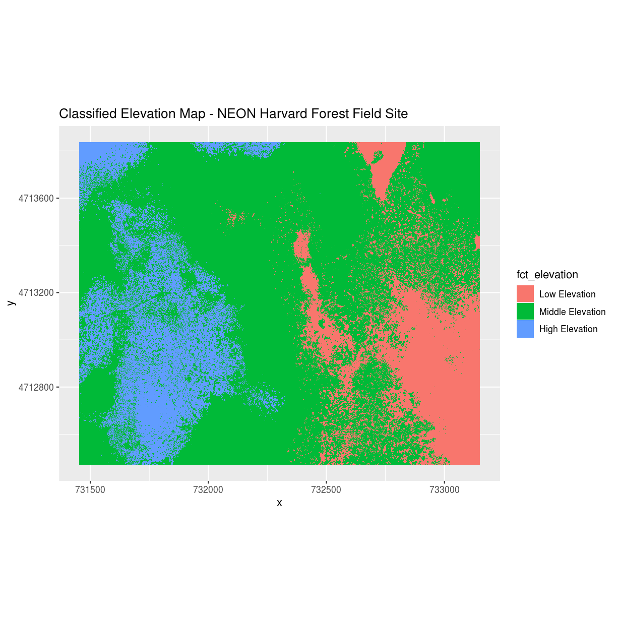
The following map shows elevation data for the NEON Harvard Forest field site. In this map, the elevation data (a continuous variable) has been divided up into categories to yield a categorical raster.

Advantages and Disadvantages

Advantages:

• representation of continuous surfaces
• potentially very high levels of detail
• data is ‘unweighted’ across its extent - the geometry doesn’t implicitly highlight features
• cell-by-cell calculations can be very fast and efficient

Disadvantages:

• very large file sizes as cell size gets smaller
• can be difficult to represent complex information
• Measurements are spatially arranged in a regular grid, which may not be an accurate representation of real-world phenomena.
• Space-filling model assumes that all pixels have value
• Changes in resolution can drastically change the meaning of values in a dataset

Important Attributes of Raster Data

A raster is just an image in local pixel coordinates until we specify what part of the earth the image covers. This is done through two primary pieces of metadata:

Extent

The spatial extent is the geographic area that the raster data covers - a bounding box defined by the minimum and maximum x and y coordinates of the data.

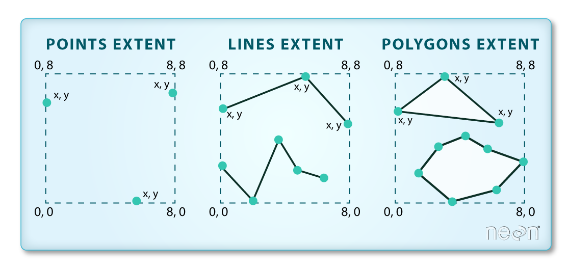
(Image Source: National Ecological Observatory Network (NEON))

Extent Challenge

In the image above, the dashed boxes around each set of objects seems to imply that the three objects have the same extent. Is this accurate? If not, which object(s) have a different extent?

Solution

The lines and polygon objects have the same extent. The extent for the points object is smaller in the vertical direction than the other two because there are no points on the line at y = 8.

Resolution

A resolution of a raster represents the area on the ground that each pixel of the raster covers. The image below illustrates the effect of changes in resolution.

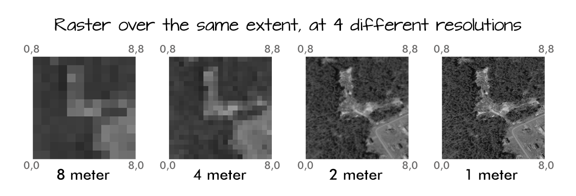
(Source: National Ecological Observatory Network (NEON))

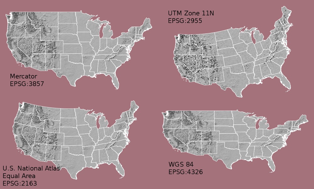
Coordinate Reference System (CRS)

This specifies the datum, projection, and additional parameters needed to place the raster in geographic space.

For a dedicated lesson on CRSs, see: https://datacarpentry.org/organization-geospatial/03-crs/index.html

Affine Geotransformation

This is the essential matrix that relates the raster pixel coordinates (rows, columns) to the geographic coordiantes (x and y defined by the CRS).

This is typically a 6-parameter matrix that defines the origin, pixel size and rotation of the raster in the geographic coordinate system:

    Xgeo = GT(0) + Xpixel*GT(1) + Yline*GT(2)
    Ygeo = GT(3) + Xpixel*GT(4) + Yline*GT(5)

You may have encountered an ESRI World file, which defintes this matrix.

For more information about the common GDAL data model used by most GIS applications: https://www.gdal.org/gdal_datamodel.html

Raster Data Format

Raster data can come in many different formats. For this workshop, we will use the GeoTIFF format which has the extension .tif. A .tif file stores metadata or attributes about the file as embedded tif tags. For instance, your camera might store EXIF tags that describes the make and model of the camera or the date the photo was taken when it saves a .tif. A GeoTIFF is a standard .tif image format with additional spatial (georeferencing) information embedded in the file as tags. These tags should include the following raster metadata:

1. Geotransform (defines extent, resolution)
2. Coordinate Reference System (CRS)
3. Values that represent missing data (NoDataValue)

Spatially-aware applications are careful to interpret this metadata appropriately. If we aren’t careful (or are using a raster-editing application that ignores spatial information), we can accidentally strip this spatial metadata. Photoshop, for example, can edit GeoTiffs, but we’ll lose the embedded CRS and geotransform if we save to the same file!

More Resources on the .tif format

• GeoTIFF on Wikipedia
• OSGEO TIFF documentation

Multi-band Raster Data

A raster can contain one or more bands. One type of multi-band raster dataset that is familiar to many of us is a color image. A basic color image consists of three bands: red, green, and blue.

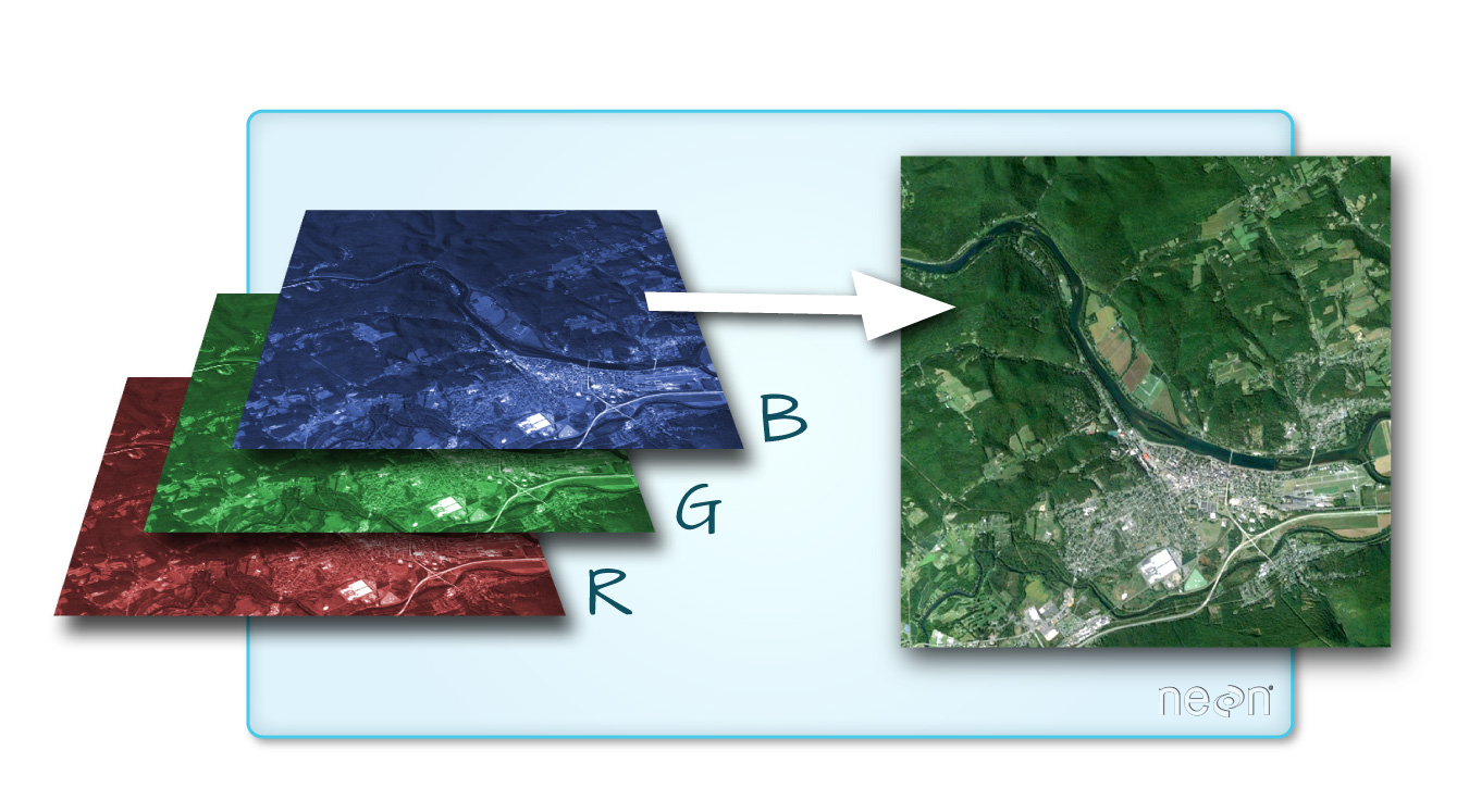
(Source: National Ecological Observatory Network (NEON).)

Each band represents light reflected from the red, green or blue portions of the electromagnetic spectrum. The pixel brightness for each band, when composited creates the colors that we see in an image.

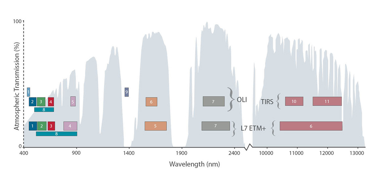(Source: L.Rocchio & J.Barsi)

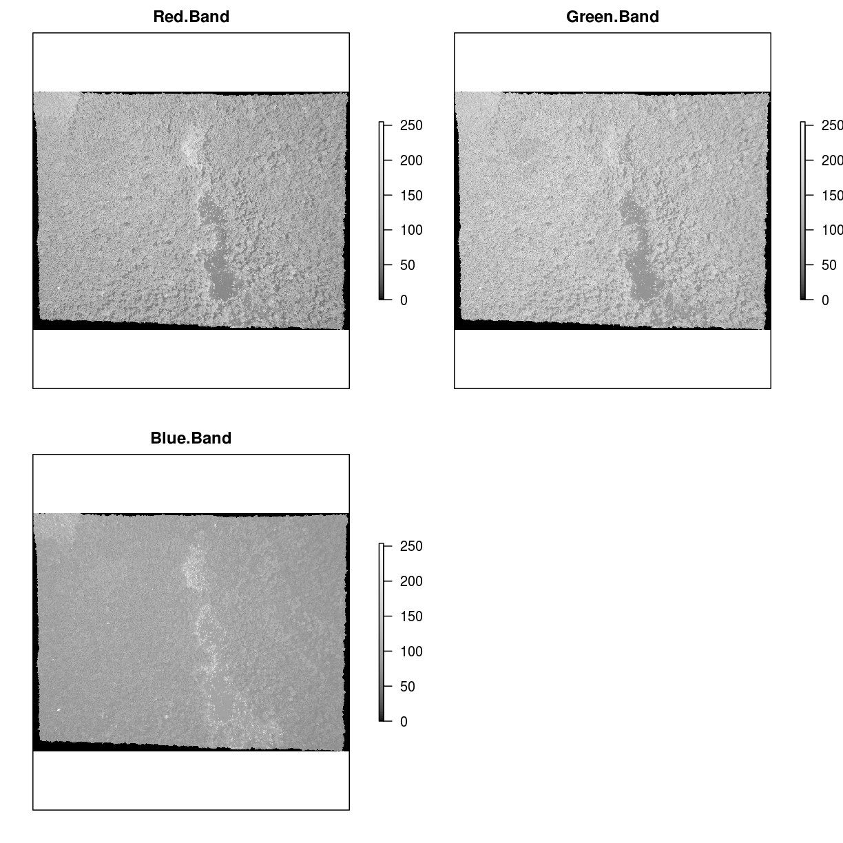
We can plot each band of a multi-band image individually.

Or we can composite all three bands together to make a color image.

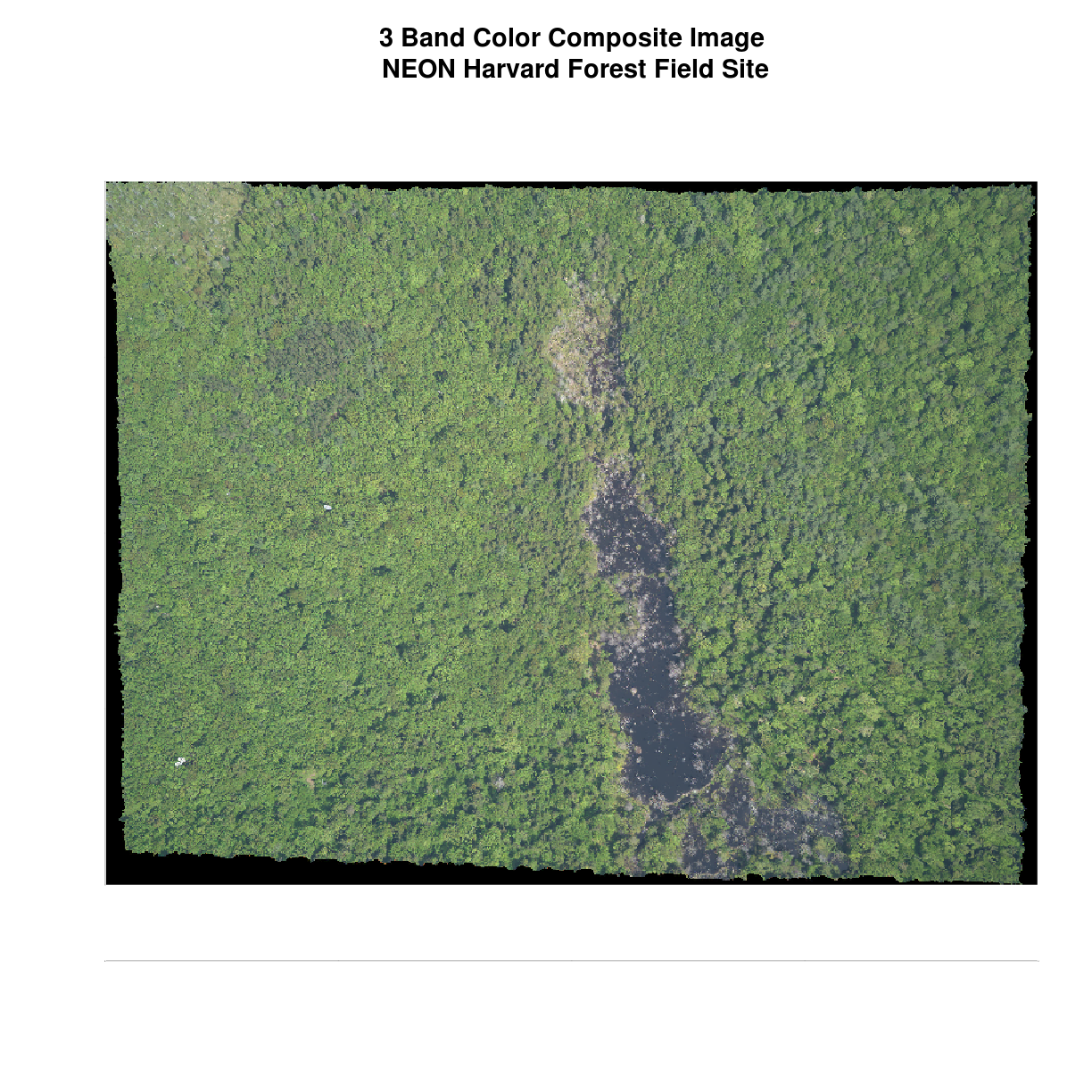
In a multi-band dataset, the rasters will always have the same extent, resolution, and CRS.

Other Types of Multi-band Raster Data

Multi-band raster data might also contain:

1. Time series: the same variable, over the same area, over time.
2. Multi or hyperspectral imagery: image rasters that have 4 or more (multi-spectral) or more than 10-15 (hyperspectral) bands

• Much of this lesson was adapted from: https://datacarpentry.org/organization-geospatial/01-intro-raster-data/index.html

Key Points

• Raster data is pixelated data where each pixel is associated with a specific location.

• Raster data always has an extent and a resolution.

• The extent is the geographical area covered by a raster.

• The resolution is the area covered by each pixel of a raster.