Overview
Teaching: 5 min Exercises: 10 minQuestions
How do I create a time series for a given location?
How can I plot that time series within Google Earth Engine?
How do I make that plot interactive?
Objectives
Load high resolution crop imagery.
Dynamically select lat/longs for creating time series plots.
Create a time series of NDVI and EVI for a selected point.
Overview
This code allows users to dynamically generate time series plots for from points that are dynamically chosen on a map on the fly. The time series show the 16 day composites of Normalized Difference Vegetation Index and Enhanced Vegetation Index at 250 m resolution. These indices are derived from MODIS.
Link to a static version of the full script used in this module: https://code.earthengine.google.com/a47b635ed6a11a99199674364afb9944
Define User Specifications
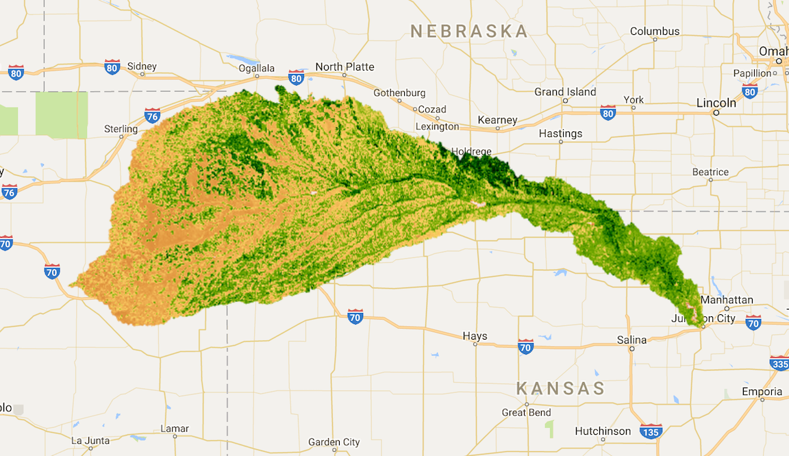
This script is structured to make it easy for the user to select different images, dates and regions. For this exercise, we are going to leave the parameters as they are to set the extent as a study area in the Midwest, the Republican River Basin
// load WBD dataset & select the Republican watershed
var WBD = ee.FeatureCollection("USGS/WBD/2017/HUC06");
Map.addLayer(WBD, {}, 'watersheds');
var setExtent = WBD.filterMetadata('name', 'equals', 'Republican');
Load High Resolution Crop Imagery
Here we are loading three different types of high resolution crop imagery. The first two datasets are already in Earth Engine. The third dataset is an Greenness index calculated from Landsat imagery. Instead of calculating the GI on the fly in this code, Jill pre-computed the index, exported the raster and is calling the pre-made raster. Practices like this can help speed up your code.
-
Cropland Data Layer (CDL) from the USDA National Agriculture Statistics Service at 30 meters resolution. This is generated annually from 2008-present. Each pixel is assigned a value that corresponds to a specific crop.
-
The National Agricultural Imagery Program (NAIP) aerial imagery from the USDA. This imagery has a 1 meter (!) ground sampling distance. This is a three band raster used to depict natural color imagery (RGB). States are imaged every 2-3 years on a rotating cycle.
-
A derived Greenness Index derived from Landsat imagery (30 m) specific to the study area. This index is computed by taking a composite of the greenest pixel, defined as the pixel with the highest NDVI, for a given time period.
// CDL: USDA Cropland Data Layers
var cdl = ee.Image('USDA/NASS/CDL/2010').select('cropland').clip(setExtent);

// NAIP aerial photos
var StartDate = '2010-01-01';
var EndDate = '2010-12-31';

var naip = ee.ImageCollection('USDA/NAIP/DOQQ')
    .filterBounds(setExtent)
    .filterDate(StartDate, EndDate);

// Derived Landsat Composites --------------------

// annual max greenness image for background (previously exported asset)
var annualGreenest = ee.Image('users/jdeines/HPA/2010_14_Ind_001')
                    .select(['GI_max_14','EVI_max_14'])
                    .clip(setExtent);
Load MODIS derived products for NDVI and EVI
NDVI and EVI are two different vegetation indices that can be calculated from red and near-infrared bands. Here we are using a derived MODIS 16 day composite product that has pre-computed bands for NDVI and EVI. You could also compute them yourself using the normalizedDifference function. Again we will filter the collection to the dates, bands and region of interest.
// add satellite time series: MODIS EVI 250m 16 day -------------
var collectionModEvi = ee.ImageCollection('MODIS/006/MOD13Q1')
    .filterDate(StartDate,EndDate)
    .filterBounds(setExtent)
    .select('EVI');

// add satellite time series: MODIS NDVI 250m 16 day -------------
var collectionModNDVI = ee.ImageCollection('MODIS/006/MOD13Q1')
    .filterDate(StartDate,EndDate)
    .filterBounds(setExtent)
    .select('NDVI');
Visualize the High Resolution imagery
Here we map the CDL, NAIP and Annual Greenest Pixel composites.
- Time Saving Tip: If you are using a public dataset, often you can find nice palettes by sifting through forum posts. Some like the CDL come with a palette embedded.
- Tip: Hexadecimal browser color picker plug-ins are helpful for figuring out which colors correspond to which codes.
- Tip:: Use the
falseargument if you want to load a layer to the map but NOT have it turned on each time you run the code.
// Visualize ----------------------------------------------------------------------------------
Map.centerObject(setExtent, 8);

// A nice EVI palette
var palette = [
  'FFFFFF', 'CE7E45', 'DF923D', 'F1B555', 'FCD163', '99B718',
  '74A901', '66A000', '529400', '3E8601', '207401', '056201',
  '004C00', '023B01', '012E01', '011D01', '011301'];

// greenest images
Map.addLayer(annualGreenest.clip(setExtent).select('GI_max_14'),
    {min:.75, max: 15, palette: palette}, 'GI - annual');

// cdl and naip
Map.addLayer(cdl, {}, 'cdl', false);
Map.addLayer(naip, {}, 'naip', false);
Create a User Interface
You can alter the client-side user interface (UI) through the ui package by adding widgets to the Code Editor interface. You can read about the ui package in the UI Overview section of the Developers Guide
The general idea is that you make a widget, which could be simple (a button) or complex (a chart). Then you define the behavior of the widget and then add it to the display. Here we create a panel, define the contents of the panel using labels, and create a callback function so the user can click a point and it will record the lat/long as an object called points. You can read more about how to define the panel and layouts in the Panels section of the Developers Guide.
// Create User Interface portion --------------------------------------------------
// Create a panel to hold our widgets.
var panel = ui.Panel();
panel.style().set('width', '300px');

// Create an intro panel with labels.
var intro = ui.Panel([
  ui.Label({
    value: 'Two Chart Inspector',
    style: {fontSize: '20px', fontWeight: 'bold'}
  }),
  ui.Label('Click a point on the map to inspect.')
]);
panel.add(intro);

// panels to hold lon/lat values
var lon = ui.Label();
var lat = ui.Label();
panel.add(ui.Panel([lon, lat], ui.Panel.Layout.flow('horizontal')));

// Register a callback on the default map to be invoked when the map is clicked
Map.onClick(function(coords) {
  // Update the lon/lat panel with values from the click event.
  lon.setValue('lon: ' + coords.lon.toFixed(2)),
  lat.setValue('lat: ' + coords.lat.toFixed(2));
  var point = ee.Geometry.Point(coords.lon, coords.lat);
Add the time series plots to the panels
Now that we have set up our user interface and built the call-back, we can define a time series chart. The chart uses the lat/long selected by the user and builds a time series for NDVI or EVI at that point. It takes the average NDVI or EVI at that point, extracts it, and then adds it to the time series. This series is then plotting as a chart.
  // Create an MODIS EVI chart.
  var eviChart = ui.Chart.image.series(collectionModEvi, point, ee.Reducer.mean(), 250);
  eviChart.setOptions({
    title: 'MODIS EVI',
    vAxis: {title: 'EVI', maxValue: 9000},
    hAxis: {title: 'date', format: 'MM-yy', gridlines: {count: 7}},
  });
  panel.widgets().set(2, eviChart);

  // Create an MODIS NDVI chart.
  var ndviChart = ui.Chart.image.series(collectionModNDVI, point, ee.Reducer.mean(), 250);
  ndviChart.setOptions({
    title: 'MODIS NDVI',
    vAxis: {title: 'NDVI', maxValue: 9000},
    hAxis: {title: 'date', format: 'MM-yy', gridlines: {count: 7}},
  });
  panel.widgets().set(3, ndviChart);
});

Map.style().set('cursor', 'crosshair');

// Add the panel to the ui.root.
ui.root.insert(0, panel);
You should see something like this appear in the bottom left:
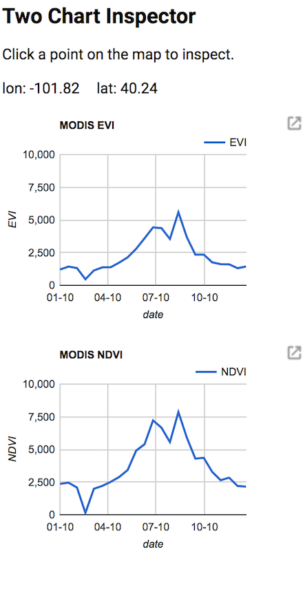
Exploring the NDVI and EVI plots for different crop types.
Toggle the Greenness, CDL and NAIP imagery layers on and off. Use the inspector to click on pixels with different levels of Greenness or different crop types and explore the differences in the NDVI time series between different pixels.
Extracting Time Series Data for larger regions or more points
If you are computing the indices on the fly, or you have many points or areas of interest, you may have the unpleasant experience of your code timing out. One way to avoid that is to just export the time series as a .csv to Google Drive or Cloud Storage. An example of how to do this can be found in Episode 04: Reducers of this tutorial.
Key Points
Time series data can be extracted and plotted from Image Collections for points and regions.
GEE has increasing functionality for making interactive plots.
The User Interface can be modified through the addition of widget.